Linear Regression in R
Implementing Linear Regression
Using the closed form formula for beta minimizing the mean squared error (MSE):
$\hat{\beta} = (X^TX)^{-1}X^TY$
linear <- function(y, X) {
# fit a linear model
beta <- solve(t(X) %*% X) %*% t(X) %*% y
return(beta)
}
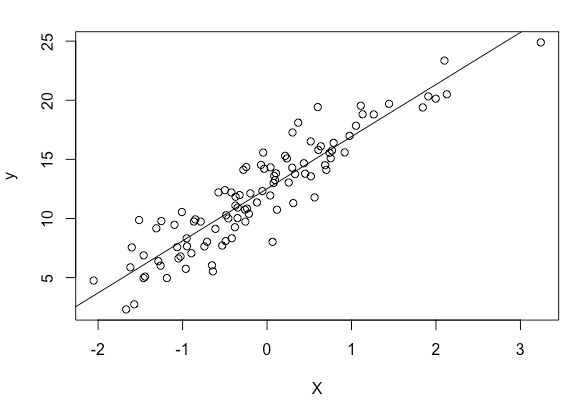
# simulate some data:
n <- 100
X <- rnorm(n)
# the "true" function plus Gaussian error:
y <- 4.5*X + 12.345 + rnorm(n, 0, 1) * 2
plot(X, y)
# augment X with a column of 1's
X <- cbind(X, rep(1,n))
# fit the model
beta = linear(y, X)
# plot the fit line
X <- -10:10
y <- beta[1] * X + beta[2]
lines(X, y)
Using lm For Fitting Linear Models
lm is used to fit linear models. Type ?lm in RStudio for help and documentation.
For the above example, model <- lm(y ~ X) will fit a linear model to the data.
Another example: prostate cancer dataset. The description of the dataset can be found here.
> dat <- read.table('prostate.data')
> head(dat)
      lcavol  lweight age      lbph svi       lcp gleason pgg45       lpsa train
1 -0.5798185 2.769459  50 -1.386294   0 -1.386294       6     0 -0.4307829  TRUE
2 -0.9942523 3.319626  58 -1.386294   0 -1.386294       6     0 -0.1625189  TRUE
3 -0.5108256 2.691243  74 -1.386294   0 -1.386294       7    20 -0.1625189  TRUE
4 -1.2039728 3.282789  58 -1.386294   0 -1.386294       6     0 -0.1625189  TRUE
5  0.7514161 3.432373  62 -1.386294   0 -1.386294       6     0  0.3715636  TRUE
6 -1.0498221 3.228826  50 -1.386294   0 -1.386294       6     0  0.7654678  TRUE
# split into training and test set
x <- sample(rep(1:8,each=12))
dat.tr <- dat[x != 1,]
dat.te <- dat[x == 1,]

# fit a full model with all features
full <- lm(lpsa ~ ., data=dat.tr)
# training error
tr_err.full <- predict(full)
with(dat.tr, mean((lpsa - tr_err.full) ^2))
# test error
pr.full <- predict(full, newdata=dat.te)
with(dat.te, mean((lpsa - pr.full) ^2))

# fit a reduced model with a subset of features
reduced <- lm(lpsa ~ lcavol + svi + lcp, data=dat.tr)
# training error
tr_err.reduced <- predict(reduced)
with(dat.tr, mean((lpsa - tr_err.reduced) ^2))
# test error
pr.reduced <- predict(reduced, newdata=dat.te)
with(dat.te, mean((lpsa - pr.reduced) ^2))
> full

Call:
lm(formula = lpsa ~ ., data = dat.tr)

Coefficients:
(Intercept)       lcavol      lweight          age         lbph          svi          lcp
   0.629841     0.575148     0.568766    -0.024590     0.094223     0.691748    -0.128993
    gleason        pgg45
   0.032534     0.005683

> reduced

Call:
lm(formula = lpsa ~ lcavol + svi + lcp, data = dat.tr)

Coefficients:
(Intercept)       lcavol          svi          lcp
     1.4460       0.6227       0.6470      -0.0394